A few Python dictionary optimizations

There are a few interesting tricks that Python uses to implement dictionaries/hash tables that I recently learned about, so I thought it might be worthwhile to write things down.

Compact Dictionary Structure

The original Python dict implementation stored information in a sparse table of (hash(key), key, value) tuples, e.g.,

d = Dict()
d.insert("how's", 0)
d.insert("it", 1)
d.insert("going", 2)
print(d)
"""
[
  ('--', '--', '--'),
  (1661004076365885705, "how's", 0),
  (-4153333719876124694, 'going', 2),
  ('--', '--', '--'),
  ('--', '--', '--'),
  ('--', '--', '--'),
  (8217317223982075798, 'it', 1),
  ('--', '--', '--'),
]
"""

where each row is allocated 24 bytes of memory. The table is kept sparse to avoid too many collisions upon insertion–every time the table gets more than two-thirds full, it’s resized. This results in a table that uses 24 * t bytes of memory (where t is the table size), even though only n << t rows are actually occupied.

To avoid this inefficiency, Python 3.7+ instead separates the hash table into a dense key-value table which contains the (hash(key), key, value) tuples that have been inserted into the dict and a sparse index table which contains the indices into that key-value table. For example:

d = CompactDict()
d.insert("how's", 0)
d.insert("it", 1)
d.insert("going", 2)
print(d)
"""
IndexTable:
[
  None,
  0,
  2,
  None,
  None,
  None,
  1,
  None,
]

KVTable:
[
  (1661004076365885705, "how's", 0),
  (8217317223982075798, 'it', 1),
  (-4153333719876124694, 'going', 2),
]
"""

This structure takes up 24*n + sizeof(index)*t bytes, which can reduce memory usage by 30-95% in practice. Furthermore, it makes iteration through dictionary elements faster, since the previous implementation would loop over all of the rows of the sparse hash table, while the new version only needs to iterate over the dense key-value table. It also makes resizing faster, since only the index table needs to be reconfigured.

Probing with Perturbation

Once we’ve computed a key’s hash, how do we find the appropriate index in the table for insertion or retrieval? If our table is of size t, to convert the hash into an index that fits within the table limits, it’s common to use a binary mask that grabs the last log2(t) significant digits of a hash h. For example if t = 8 and h = 5123 = 0b1010000000011, we can use the mask 0b111 and do a bitwise &: 0b1010000000011 & 0b111 = 0b011 = 3.

What do we do if this bucket is already occupied? Maybe the simplest approach is to do linear probing, which just looks in the next bucket, and the next one, and so on until it finds one free:

def linear_probe(hashtable: list[tuple[Any, Any, Any]], key_hash: int) -> int:
    """classic linear probing: probe one bucket at a time from the initial index until an empty
    spot is found
    """
    table_size = len(hashtable)
    # binary mask of all 1s
    mask = (1 << int(math.log2(table_size))) - 1
    idx = key_hash & mask
    while hashtable[idx][0] not Empty:
      idx = (idx + 1) % table_size
    return idx

One problem with linear probing, however, is that it can easily result in clumping, wherein a lot of occupied buckets end up next to each other, and insertions may take O(n) rather than O(1). For example, if the hashes for two different keys have the same last log2(t) significant bits, they’ll try the same buckets in the same order.

To avoid this issue, Python uses an approach called “linear probing with perturb,” which takes into account higher order bits to generate the probe trajectory:

def linear_probe_perturb(hashtable: list[tuple[Any, Any, Any]], key_hash: int, perturb_val: int = 5) -> int:
  """a more sophisticated probing approach based on Python's approach
  
  rather than just probe one spot at a time from the initial index, right-shift the hash key and use that to generate the 
  next bucket to check. this allows the process to take into account the higher-order bits of the hash. 
  """
  table_size = len(hashtable)
  mask = (1 << int(math.log2(table_size))) - 1
  idx = key_hash & mask
  perturb = key_hash
  while hashtable[idx][0] not Empty:
    perturb >>= perturb_val
    # guarantees that every index will eventually be visited
    idx = (5 * idx + 1 + perturb) & mask

  return idx

This method simply right-shifts the hash each step to generate the next bucket in which to look. The 5 * idx + 1 part ensures that the trajectory will traverse every bucket in the table (as long as the table size is a power of 2). Note also that when the table size is a power of 2, using the bitwise & is equivalent to % table_size but is faster because it’s only one CPU operation.

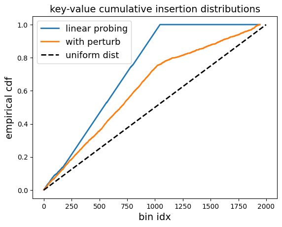
To compare the effectiveness of linear probing with and without perturbation, we can look at the entropy of the bucket allocations as we make more and more insertions to a dictionary:

d0 = Dict(linear_probe)
d1 = Dict(linear_probe_perturb)
for i in range(1000):
  key = str(uuid.uuid4())
  d0.insert(key, i)
  d1.insert(key, i)

d0_bins = [row[0] != d0._EMPTY for row in d0.hashtable]
d1_bins = [row[0] != d1._EMPTY for row in d1.hashtable]
plt.plot(np.cumsum(d0_bins) / 1000, lw=2, label="linear probing")
plt.plot(np.cumsum(d1_bins) / 1000, lw=2, label="with perturb")
xs = np.arange(2000)
plt.plot(xs, xs / 2000, lw=2, ls='--', color='k', label="uniform dist")
plt.xlabel("bin idx", fontsize=14)
plt.ylabel("empirical cdf", fontsize=14)
plt.title("key-value cumulative insertion distributions", fontsize=14)
plt.legend(fontsize=13)
plt.show()

We can see that using perturbation does in fact make the distribution of allocated buckets more uniform!

As an aside, I think the clumping problem is kind of interesting, because it’s the opposite of the issue faced in memory allocation, where contiguous blocks of allocations are desirable, and fragmentation leads to poor performance and failed allocations.

My toy Dict implementation which I used to test this stuff can be found here. Thanks for reading–hope this was interesting!