Implementing ViT in PyTorch

I’ve been trying to get a better understanding of the broader transformer-verse, so I thought it would be fun/useful to implement a Vision Transformer (ViT, Dosovitskiy et al., 2020). You can find the full implementation here.

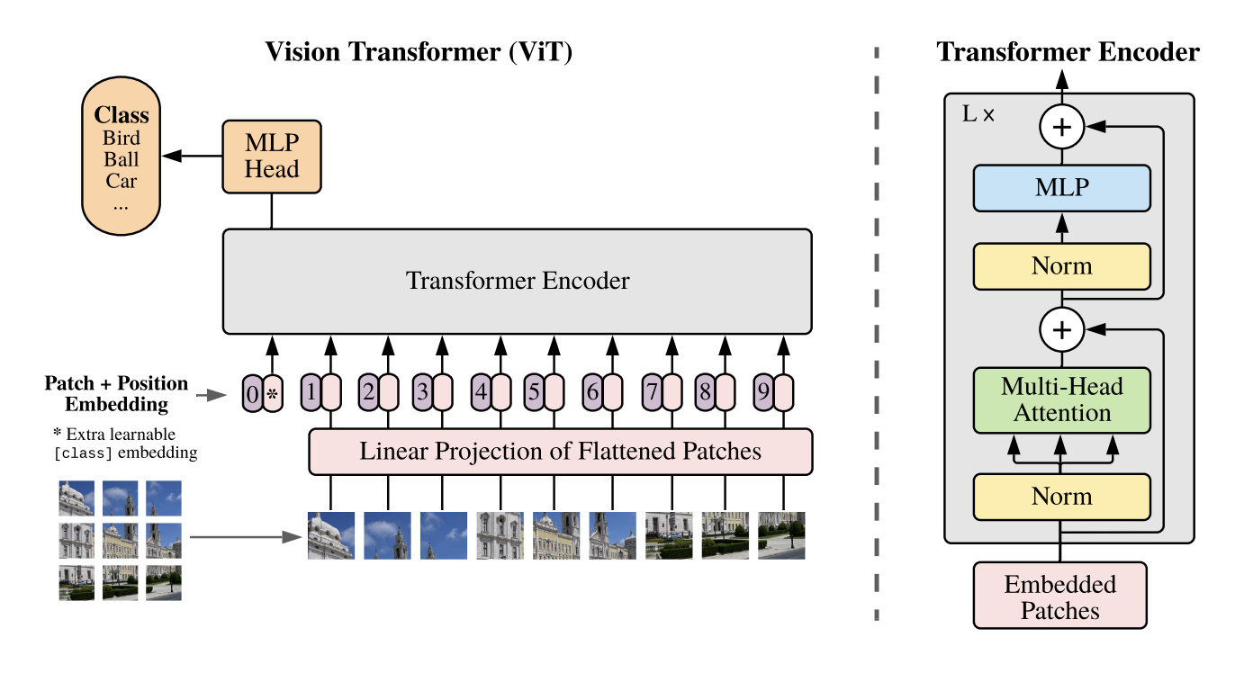
The main motivation behind ViT was to replicate transformers’ success in NLP on computer vision tasks while modifying the architecture as little as possible. To do this, ViT breaks up images into patches which are then passed through a linear embedding and treated as a 1D sequence of tokens:

At a high-level, you basically just flatten these patches and feed in the resulting sequence to your transformer in the same way you would for a language-based model. The sequence length N is therefore the number of patches and the input dimension I is n_channels * patch_size ** 2. For classification, though, there’s no masking or anything like you see in language modeling. Instead, you prepend a special learned classification token to the input sequence (making the final sequence length T = N + 1). The idea is that this token can learn to attend to all the most relevant tokens in the sequence for classification. At the top layer of the model, you add a head (either a linear layer or MLP) which takes the representation at this (first) position in the sequence and maps it to class logits:

To get a more concrete sense of what’s happening in code, here’s my implementation:

class ViT(nn.Module):

    def __init__(self, config):
        super().__init__()
        token_dim = config.n_channels * config.patch_size ** 2
        self.token_embed = nn.Linear(token_dim, config.model_dim, bias=False)
        self.pos_embed = nn.Embedding(config.seq_len + 1, config.model_dim)
        self.cls_embed_11D = nn.Parameter(0.1 * torch.ones(1, 1, config.model_dim))
        self.blocks = nn.ModuleList([Block(config) for _ in range(config.n_layers)])
        self.head = nn.Sequential(
            nn.LayerNorm(config.model_dim),
            nn.Linear(config.model_dim, config.model_dim),
            nn.GELU(),
            nn.Linear(config.model_dim, config.n_classes)
        )
    
    def forward(self, x_BNI, y_B=None):
        # add classification token and embed image tokens/patches
        B, N, _ = x_BNI.shape
        T = N + 1
        x_BND = self.token_embed(x_BNI)
        D = x_BND.shape[2]
        x_BTD = torch.cat([self.cls_embed_11D.expand(B, 1, D), x_BND], dim=1)
        # add positional embedding
        x_BTD = x_BTD + self.pos_embed(torch.arange(T, device=x_BTD.device))
        # apply blocks
        for block in self.blocks:
            x_BTD = block(x_BTD)
        # apply head on first (classification) position in the sequence
        logits_BC = self.head(x_BTD[:, 0, :])
        loss = None
        if y_B is not None:
            loss = F.cross_entropy(logits_BC, y_B)
        return logits_BC, loss

In this code, as in the paper, you can see that I just used a learned 1D positional embedding for the sequence. The paper authors didn’t find any real benefit in adding “2D”-aware positional embeddings in their experiments. This is somewhat surprising, and it’s especially impressive that ViT can get such strong performance without any of the inductive biases for images that convolutional networks have. There’s a slight caveat here, in that the main avenue for success identified by the authors is to pre-train the model on a huge amount of data and then fine-tune it on the downstream classification task of choice (sound familiar?). Yet another example of scale (model + data) producing super strong results.

In my case, I just implemented the simplest possible version of this approach for classification on CIFAR-10 (no pre-/post-training). To start, I just wanted to see the loss go down, and a simple 6-layer model starts overfitting over 20 epochs:

After this sanity check, I basically wanted to play around with the model and see if I could boost compute efficiency a bit. It was very easy to drive loss down on the training set, but overfitting was a major issue. Realistically, I think the model was just a bit too big. ViT also isn’t known for excelling on small datasets like CIFAR-10 - it seems to do a lot better with bigger images, I’m guessing that’s related to the minimum patch size required for a patch to contain useful signal. The simplest thing to do to increase GPU utilization was to bump up both the model size and the batch size. I moved the model dimension up from 64 to 192 and reduced the number of heads from 16 to 12. I also scaled the batch size up to 1024 from 128 and bumped up the learning rate at a roughly linear rate to 2e-3. Initially training on my laptop CPU took around 15-20 minutes, but making these changes and moving to an A100 allowed the network to read 99% accuracy in 40 epochs on the training set in around 3 minutes. Another factor which bumped GPU utilization and made training faster was adding more CPU workers (cores) parellelizing the PyTorch dataloaders. Moving from 2 workers to 4 and pinning the data in memory. Without this change, the GPU was processing data more quickly than it was being fed, leading to idle time.

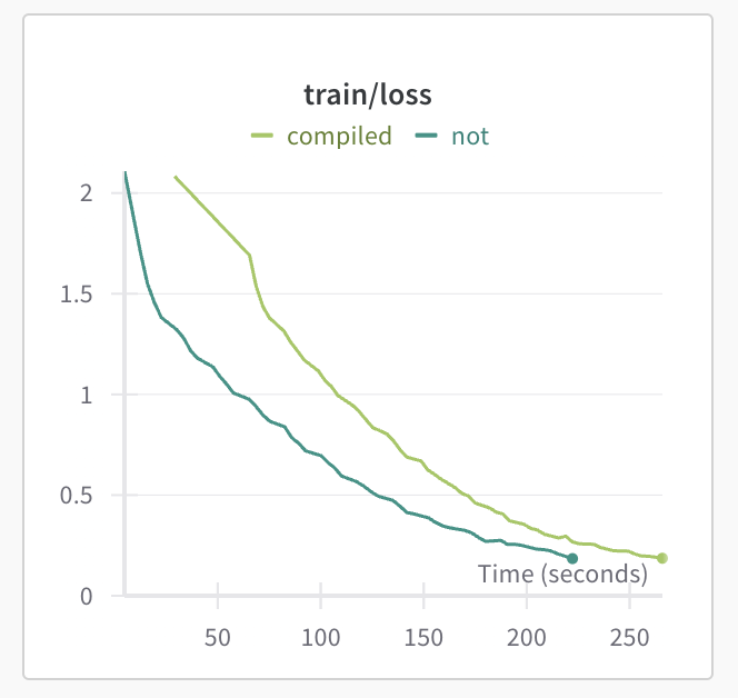
One cool feature in PyTorch 2.0 and above is the ability to compile the model to run more efficiently. This also sped up training, though for short training periods like I did, the extra time required to compile the model is not insignificant compared to the overall training time.

I also tested out automatic mixed precision (AMP) training, but again I think things are just too small in this setting for this to make a meaningful difference. Regardless, it’s worth mentioning. The idea behind AMP training is to both speed up training and reduce memory load by storing a “master copy” of the model weights in full 32-bit precision while using half-precision (16-bits) for the forward and backward passes. To avoid gradient underflow for small loss values, the loss is usally scaled up before gradient computation, then the gradients are scaled back down before being passed to the optimizer to compute updates.

scaler = GradScaler()
dtype = torch.bfloat16 if torch.cuda.is_available() and torch.cuda.is_bf16_supported() else torch.float16
optimizer = torch.optim.AdamW(
    net.parameters(),
    lr=lr,
    betas=(0.9, 0.999),
    weight_decay=weight_decay)

for epoch in range(epochs):
    running_loss = 0.0
    for i, (x_BCHW, y_B) in enumerate(trainloader, 0):
        x_BNI = tokenize(x_BCHW,  vit_config.patch_size).to(device, non_blocking=True)
        y_B = y_B.to(device, non_blocking=True)

        optimizer.zero_grad()
        with autocast(dtype=dtype):
            _, loss  = net(x_BNI, y_B)
        scaler.scale(loss).backward()
        scaler.step(optimizer)
        scaler.update()

Anyway, this was a fun exercise.